Transient behaviour and homogeneous kinetics for the widely placed double-channel electrodes: An Analytical solution. 

**Summary**

1. Introduction.

The double-channel electrode arrangement, pioneered by Gerischer [ ], is a valuable approach to the study of intermediates and products of electrode reactions. The basis of such investigations is as follows. A solution species, A, passes over the upstream generator electrode where it oxidizes (or reduces to a species B), i.e.

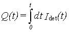
The species B is then transported to the downstream detector electrode where it is analysed amperometrically, generally via reduction ( or oxidation) back to A. The experiment is quantitatively characterized by so-called "collection efficiency", N, given by

where I_gen and I_det are currents at the generator and detector electrodes, respectively. Flow cell is usually includes an electrode of width d where d is greater than the cell's height h and a transport problem is really two dimensional. The two dimensional sketch of cells is presented on the fig.1. Matsuda et al. had calculated the steady state limiting currents for the case when thickness of a diffusion layer is significantly lower than height h of the channel:

where V_f is the volume flow rate, D is the diffusion coefficient of species B and  is the maximum linear characteristic length ( = _gen + _gap + _det ). When condition (2) is fulfilled, the velocity near the wall can be linearazed and Leveque -type solution is applicable. In the other case when the parameter in the right side of (2) is of the order of unity the numerical solutions for Poiseuille flow have been performed by Compton and coworkers [ ].

In present paper we are going to analyze only the case of widely placed electrodes, when  _gap >> _gen, _det which is typical for the microelectrodes technique [ ], but it can be met for ordinary double electrodes as well. Taking into a account of conditions (2) allows us to use Leveque approximation in the region of the gap. Thus approximations give us the possibility to obtain the simple analytical expressions for the transient behaviour, including the time delay of current I_det after switching on I_gen and the characteristic slop of chonoamper curve. The general solution is not restricted by conditions on the Peclet numbers (based on the electrodes lengths), therefore the lateral diffusion can be taken into account if necessary. Moreover, it has been shown that features of electrode reactions on the generator electrode ( reversible or irreversible reactions, applied potential, electrode length, etc.) has no influence on the collection efficiency. Our approach can be extended on the more complicated system, for example, for the system with the first order homogeneous reactions the steady-state current efficiency has been calculated. Some particular cases, when solution is not restricted by conditions (2), are discussed.

Problem statement.

The transport process in the double-channel electrode cell can be subdivided into three stages:

(i) Transport of species A towards the surface of the generator electrode and then the transport of the product of the electrochemical reaction B out of the electrode region;

(ii) Transport of B along the gap;

(iii) Transport of B towards the surface of the detector electrode.

Because the gap is much longer than electrodes:  _gap >> _gen, _det the characteristic time of the second stage is much greater than the other ones. Therefore, two significant simplifications could be taken into account. Firstly, the convection- diffusion equations can be solved separately for each stage, even if lateral diffusion for (i) and/or (iii) is taken into account. Secondly, the transient behaviour of the system is determined only by transport along the gap and we can use the steady-state solutions in the vicinity of electrodes.

Further we will use mainly nondimmensional variables, using notations with a hat for the dimensional ones. The value of σ^{-1 will be the unity of time t=}σ  , where

is a gradient of fluid velocity near the wall: v_x=σ . The value (D/κ)^1/2 will be used as a unity of distance:

In this notation the Peclet number, associated with the length  is simply l². The concentration of [A] at infinity will be used as a scale for concentrations; dimensionless current

where F is a Faraday number.

The sub-problem (i), i.e. steady state convection-diffusion transport towards the channel electrode is well studied [ ]. For high Peclet number l² >>1 the classic Leveque solution is valid:

For small Peclet number l<<1 Ackerberg et al. had derived the expression

In the case of different diffusion coefficients of A and B the actual form of (6), (7) depends on the choice of dimensionless variables in (4) and (5). If D_B has been chosen, the right-hand sides of (6) and (7) must be multiplied by factor D_B/D_A and the value of l must been correct correspondently.

Newman [ ] calculated numerically the current-Peclet number dependence for all Peclet numbers, including l~1. Perdley [ ] has investigated several-terms approximations and find out that none of them works at l~1 satisfactorily. He has also shown that it is better to use Leveque expression (6) for all l>1 rather than another ones which take into account the lateral diffusion. In series of the works by Compton and coworkers [ ] investigated numerically the cases of reversible and irreversible electrode reactions.

The sub-problem (ii) is described by diffusion-convection equation for nondimensional concentration c of species B:

in the area t>0, y>0, x>0. The initial and boundary conditions are:

where δ_{+(x) is Dirak's function. The boundary conditions (10) and (11) correspond to absence of species B in the bulk of the solution. The boundary condition (12) describes that the only source of substance B is of a small size and placed at the beginning of the coordinate system generating, starting from t=0, the permanent electrical current I}gen. Solution of the system (8)-(12) gives us the concentration distribution c(t,x,y) and, in particular, c(t,L,0) near the electrode.

Solution of the subproblem (iii) is absolutely analogical to that of the problem (i). The size of the diffusion layer at x» L is far above the length of the detector electrode, therefore the test electrode has no influence on the concentration distribution within the diffusion layer. Really, we have the second channel electrode which is situated in the bulk solution of dimensionless concentration c(t,L,0) contrary to the concentration for the generator electrode being equal unity. The expression for the collective efficiency is

In order to find the final expression for N we have to solve the system (8)-(12). The reader interested only in the final results can skip the next section.

Solution of the transport equation for the gap region.

The double Laplace transformation of expression (8) firstly with respect to t ( transform variables s) and secondly with respect to x ( transform variables p) gives:

where  denotes the double-Laplace transformation of variable c. The solution of (14), which satisfies the boundary and initial conditions (9)-(11) can be found in the form:

where Ai[z] denotes the Airy function [Ambramovitz, Stegan] and the constant factor must be obtained from Laplace transformation of (12):

Combining (15) and (16), we obtain the concentration distribution at y=0

where

In order to find the inverse Laplace transformation of (17) we have to simplify it, substituting the Taylor series for f[z]. Considering that according to the definition of Airy function Ai"[z]=zAi[z] we can obtain the useful relation

which allows us to find first several terms of series:

where

Substituting (20), (21) into (17) and taking the formal inverse Laplace transformations with respect to time and coordinate x, we obtain at y=0:

The first term in the exp.(22) corresponds to steady-state concentration. Substituting it into (13) we obtain the steady state current efficiency N₀

where I(l_det) is given by (6) or (7).

The interpretation of the second and third terms in (22) cannot be done in the same straight forward manner. For example, the second term includes the Dirak's function, i.e. formally concentration is infinitely negative at the initial time, which has no physical meaning. To find the answer we should realize that expression including Dirak's function or/and its derivatives is not truly mathematical function and must be first integrated sufficient number of times.

In fact the second term indicates that some "losses" (comparing to steady state) in current on the detector electrode occur after the generator had been switched on. The most natural thing to do is to interpret this process as a step-like one, when the current on the detector electrode is switched on at a moment t=t₀ (see Fig.2). The integration of the two first terms of (22) with respect to time gives us the time t₀, when the concentration at first time becomes nonnegative (c=0):

The mathematical background of this operation is the following. The time-dependence of charge (which passes trough the detector electrode)   is a kind of smooth

curve starting at zero (see Fig.2b) The first two-term approximation (23) gives us the straight line, which fits perfectly at a long time t>>1, but deviates significantly at the beginning. Therefore, we have to correct the approximate straight line, at least on the segment (0, t₀ ) when it becomes negative.

The second term of (22) is responsible for the "delay" and we can guess that the third (and the following ones, if necessary) give more details about a shape of the curve I_det(t). Thus, if we take some reasonable approximation for I_det(t), for example, as arctan, three terms in (22) give us the steady state current, the time delay t₀ and the speed of current changes near the time t=t₀. We are not pretending to describe an exact form of the curve, therefore we are going to take the simplest model form for I_det(t) (see fig.3a): the electric current I_det being zero up to time t₁, then changing linearly to the steady state value.

Integrating the expression (22) twice with respect to time we obtain for x=L

Analogically, the test-curve (Fig.3a) must also be integrated twice. The initial segment 0<t<t₁ is not getting changed by thus operation, while the straight line t>t₂ becomes a part of the parabola (25). The segment between points t₁ and t₂ is transformed into cubic parabola, which should meet the previous parts at the points t₁ and t₂. Moreover, at the points t=t₁ and t=t₂ the derivatives and the second derivatives of the function ò ò dtc must also be continuous. Those in total six conditions give us the system of algebraic equations for four numbers, describing the cubic parabola and the values t₁, t₂. An elementary but also rather cumbersome solution of this system gives us the simple expression for the chronoamper curve between points t₁ and t₂:

The expression (26) is valid only while the term in the square brackets in the right side is within the interval of 0 and 1.

Results and discussion.

The time dependence of collective efficiency N after calculation of constants in the expressions (22), (24), (26) (see also fig.3a) is

where t₀ is the time when N has a half value of its steady state value:

and N₀ is a steady state current efficiency

In two particular cases of high and small Peclet numbers the expression (29) can be simplified, after taking into account either (6) or (7):

Expressions (27)-(31) are given in the dimensionless form, therefore it is useful to discuss them depending on system parameters. First of all, the concentration in the diffusion layer and I_det are proportional to the current, generated by the generator electrode, therefore the collective efficiency does not depend on a size of the generator electrode, reversibility of reaction on it, the bulk concentration of substance A, its diffusion coefficient D_A and other details. Actually, these features follow directly from the assumption l_gen << l_gap » L.

For the Peclet number l²_det >>1 it is possible to neglect the lateral diffusion in the vicinity of the detector electrode and steady state collective efficiency N₀ depends only on a ratio of a length of the detector electrode l_det and a gap length l_gap» L. Therefore it does not really depend on the other system parameters, including the velocity of liquid and the diffusion coefficient. Expression (30) can also be obtained as a limiting case of Matsuda's [ ] results for l_det <<L.

In the opposite case of a very short detector electrode l²_det<<1 (exp.31) N₀ becomes dependent on L and l_det separately. Note that L and N₀ were normalized on the length (D/σ)^1/2, i.e. depending on the diffusion coefficient and fluid velocity. The value N₀ depends on the length of the system L in a standard for Leveque solution form, as L^-2/3 (compare with (30)). The dependence on the electrode length is logarithmic, i.e. rather weak.

The time period when current I_det reaches the half of its steady state value is given by a very simple expression (28). According to the expression (28), the value t₀ does not depend on the length of the detector electrode and other details of kinetics on the detector electrode. In the dimensional form it appears as

The only parameter in (32) which cannot be measured directly is the diffusion coefficient D. Therefore, expression (32) can be used for estimation of the diffusion coefficient of product B.

Finally, the expression (27) shows that the system tends to the stationary regime rather sharply: the time of transient behaviour comes to 90% of t₀. Moreover, this relative time of 90% is standard for any system. It means that after renormation by some standard value of N₀ and t₀, all N(t) must be approximately the same. Such an operation can be used to check applicability of presented theory to the real system, when the main theory assumption (l_gap>>l_det, l_gen) and absence of homogeneous reactions in the gap are in doubts.

The technique of analytical solution developed in this paper can be applied to some similar problems. For example, suppose that we are looking for current efficiency at a steady state in the system where substance B can participate in the first order homogeneous reaction, transformed into electropassive substance. The diffusion-convection equation for such a system differs from eq.(8) only by the left-hand side:

where k is a dimensionless constant of the reaction: k =  /σ .

To solve equation (33) with the boundary and initial conditions (9)-(12) we can make a Laplace transformation with respect to coordinate x only (transform variable p) and obtain the equations in the form (14), where variable s is changed for k. The transformed boundary condition (12) becomes simply _ /_y =I_gen at y=0 and Laplace transformation for the concentration at y=0 appears as

Substituting approximate expression (20) for f[z] into (34) and taking the inverse Laplace transformation, we obtain the final expression for current efficiency in a form very similar to exp.(22):

The subscript "2" of N denotes that terms of expansion for function f[z] were taken into account up to the second power. The first term in the right-hand side of (34) is N₀ (see exp.(29)-(30)) - which corresponds to a steady state in the absence of homogeneous reaction. The second term describes the main deviation of N due to a homogeneous reaction. Note that this term does not depend on a distance between the electrodes, which means that the main current efficiency "loses" happen near the generator electrode, where concentration of B is significantly higher than in the diffusion layer in general, which is described by the last term in the expression (34). The feature of the weak dependence on the homogeneous reaction in the diffusion layer reflects the fact that the detector electrode measures only a small part of the diffusion layer and that the reaction in the "bulk of diffusion layer" is not as significant as the reaction on its "leading edge".

Actually, the expression (34) is a series with respect to small parameters (k/L^2/3)<<1 and in most cases the last term can be omitted. Suppose that after "switching on" the homogeneous reaction the current efficiency changed from the value N₀ to some other value N₁. From expression (34) we can find the constant of the reaction in the linear approximation (dimension variables):

If the diffusion coefficient is known (for example, from data for t₀), expression (36) gives the possibility to compute the rate constant  . We have to note that, strictly speaking, the expression (36) is valid only for relatively slow reactions, i.e. when N₀ -N₁ <<N₀ .

Finally let us discuss the situation, when the conditions (2) is broken, i.e. thickness of the diffusion layer becomes comparable with semi-height of channel. For a rather slow flow the approximation radically different from (2) can be useful: V_fh << D  d. Under such an assumption the steady-state concentration [B] becomes uniform in the whole channel and is defined only by I_gen and the channel size h:

Therefore, the current efficiency N₀ must be calculated from

instead of (29). Of course, this value is rather small (note that the last term also depends on fluid velocity for slow flows and its measuring can bring a serious experimental difficulty. An approximate expression for the "relaxation time" t₀ for such a system can also be obtained analytically, but this problem is out of the frames of this paper.

Experimental test

Materials

Double channel experiments were conducted using 4 x 10^-3 M N,N,N',N'-tetramethyl-p-phenylenediamine (TMPD) in 0.2 M KCl solutions The TMPD was 98 percent pure (Aldrich, Steinheim) and the KCl was AnalaR (BDH, Dorset). The solutions were made with Elgastat (High Wycombe, Bucks) UHQ grade water with a resistivity not less than 18 MΩ.

The Flow Cell and Flow System

The channel flow cell and flow system have been described previously [1, 2, 3] and so only a brief description will be given here. Experiments were carried out in a flow cell fabricated in Perspex. The channel was 6 cm long , 0.6 cm wide and approximately 0.1 cm deep. The exact depth of the cell was determined from the slope of a Levich (transport limited current versus (flow rate)^1/3) [4] obtained from TMPD which has a known diffusion coefficient 6.3 x 10^-6 cm^-2 s^-1 [5]. In the experiments conducted the cell height was measured in this manner as 0.0882 cm.

The cell coverplate bore the generator and detector electrodes. The electrodes consisted strips cut from Platinum foil, 0.0255mm thick (99.95%, Goodfellows, Cambridge, UK). The electrodes were cemented to the coverplate using Araldite. The mounted electrodes were polished to a mirror finish using progressively finer diamond lapping compounds (Engis, Maidstone). The smallest diamond grit used was 0.25 μm. The dimensions of the electrodes and the gap between them were measured with a travelling microscope (see table 1). The channel cell was formed by clamping the coverplate over the channel. A silver wire pseudo-reference electrode was locate upstream of the channel and a platinum gauze counter electrode was situated immediately downstream.

Solution deoxygenated with Argon was gravity fed to the cell from a glass reservoir via several metres of 1.5mm bore glass tubing. Flow rates over a wide range (10^-1 to 10^-4 cm³ s^-1) were attained by switching between capillaries with different internal bores and by varying the height of the reservoir relative to the outlet dropper. The cell and approximately 1 metre of tubing were located in an air thermostatted box at 25 ± 0.5 ^oC.

Comparison of Theory and Experiment Results.

The dependence of t₀ versa flow velocity V_f in the power -2/3 is presented on the fig.4. Taking the value for the diffusion coefficient D=6.3 10^-6 cm² s^-1 we obtained from (32) that for the presented cell geometry this dependence must be linear with the slop equal 1.227. The real experimental value for the slop obtained by method of minimum square deviation gives us the value 1.212. Note that   in (32) has the meaning of distance between electrodes, which for the electrodes of final length define as ( _gen + _gap ) ±  _det , i.e. with accuracy of ± 7% in present case. We have taken as the  the approximate distance between middle of electrodes  =1.5 mm, which give us the real accuracy somewhat 1.2%.

On the fig.5 the example of dependence I(t) for the V_f =0.0412 cm³s^-1 is given. It has the shape of semi-wave. On the same picture the theoretical dependence (26) is given by dash-line. As was been expected the theoretical line is in the good agreement with the experimental one. Note, that theoretical line does not correspond to the slop of the real curve in some point but it is some integral characteristic. For the curves which is symmetrical in respect to the point t₀ the line (26) is goes in such way that areas I and II on the left and on the right of it appears to have the same value. At such conditions the values of areas III and IV also turn to be same. In the general case, as it was shown on the Fig.5, holding of this two conditions for two couples (I & II) and (III & IV) are imposable and the theoretical line has to balance the ration between this areas in somewhat more complicate manner.

Strictly spiking, the same idea must be used to determination of t₀ - the line t = t₀ must balance the area up and down of the experimental curve (see fig.2a). But for the most cases the nonsymmetry of the I(t) does not influence on this stage, therefore for the practical use we can identify t₀ with the time when I(t₀) =0.5 I(t® ¥ ).

*****Conclusion****

Table 1: Dimensions of cell used in double channel experiment.

References

1. B.A. Coles, R.G. Compton, J. Electroanal. Chem. 144 87 (1983).

2. R.G. Compton, P.R. Unwin, Phil. Trans. R. Soc. Lond. A 330 1 (1990).

3. R.G. Compton, G.M. Stearn, P.R. Unwin, A.J. Barwise, J. Applied Electrochem. 18 657 (1988).

4. V.G. Levich Physicochemical Methods (Prentice-Hall, Englewood Cliffs, N.J. 1962)

5. G. Harland, R.G. Compton, J.Coll. Interface Sci. 131 83 (1989).

Pedley T.J. The fluid mechanics of large blood vessels Cambr. monogr. on mech. and applied math.). Cambr.&c. 1980.

Ackerberg R.C., Patel, R.D. & Gupta, S.K. (1978) The heat/mass transfer to a finite strip at small Peclet numbers. J.Fluid Mech. 86, 49-65.